kmeans

所在包：stats包

1. 理论

算法简介

选择K个点作为初始质心
repeat
将每个点指派到最近的质心，形成K个簇
重新计算每个簇的质心
until 簇不发生变化或达到最大迭代次数

算法伪代码：

List K_means(DataSet S, int k)  {  
    List new_centrio_list = Select_init_centriole(S, k); // 选取初始的k个中心点  
    do {  
        centrio_list = new_centrio_list;  
        foreach (s in S) {  
            best_centri->distance = MAX;  
            best_centri->class = Undefine;  
            foreach (centri in centrio_list) {  
                double distance = Calculate_distance(s, centri);  
                if(best_centri->distance > distance) {  
                    best_centri->distance = distance;  
                    best_centri->class = centri->tag;  
                }  
            }  
            category_list[best_centri->class].Add(s);  
        }  
        new_centrio_list = Relocate_centriole(category_list, centrio_list, k);  
    } while(!Is_centrio_stable(new_centrio_list, centrio_list));  
    return category_list;  
}

1. 时间复杂性：O(nkt)，其中n=|S|，t为迭代的次数。每次迭代均要计算S中的每个样本同每个中心点的距离，然后将其归类为最小距离的中心点。
2. Select_init_centriole(S,k)函数是初始种子的选择，传统的K-means算法采用的爬山法，初始种子的选择决定了最后收敛的效果，现在有多种方法选择种子值。同时k的设定，在k未知时，如何自动选择k值，现在也已经有了很多方法。
3. Calculate_distance(s,centri)函数用于计算两个样本点之间的距离。距离的计算方法有很多种，最常用的距离计算公式是用阿几里德距离，但是这不一定是最优的选择。因此，距离计算也是K-means算法中需要探讨的一个问题。
4. Relocate_centriole(category_list,centrio_list,k)函数用于重置中心点。重置的方法主要有两种：k均值和k中心点。前者是将划归的各个类属样本的均值作为新的中心点，而后者是选择各个类簇的中心样本作为新的中心点。后者一般情况下具有更高的容错能力，对于噪点和离群点有更好的容错力。
5. K-means算法对离群点和噪声是非常敏感的，因此需要考虑一些策略对噪声和离群点进行处理。

   注：伪代码Ref:http://blog.csdn.net/tangbin330/article/details/8677130

欧几里得距离 euclidean metric.

sqrt(sum((x_i - y_i)^2)).

余弦相似度 余弦相似度用向量空间中两个向量夹角的余弦值作为衡量两个个体间差异的大小。相比距离度量，余弦相似度更加注重两个向量在方向上的差异，而非距离或长度上。

$$ \cos{\theta} = \frac{ \vec{x} \cdot \vec{y} } {||x|| \cdot ||y||} $$

SSE SSE（Sum of Squares for Error）误差项平方和，反映误差情况.

SSE（Sum of Squares for Error） = RSS (residual sum of squares)。

缺点： 对极端值敏感。

2. 官方示例

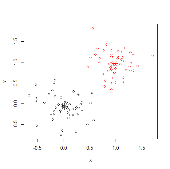
require(graphics)

# a 2-dimensional example
x <- rbind(matrix(rnorm(100, sd = 0.3), ncol = 2),
           matrix(rnorm(100, mean = 1, sd = 0.3), ncol = 2))
colnames(x) <- c("x", "y")
(cl <- kmeans(x, 2))
plot(x, col = cl$cluster)
points(cl$centers, col = 1:2, pch = 8, cex = 2)

3. iris示例

ref:http://blog.csdn.net/yucan1001/article/details/23123043

newiris <- iris;  
newiris$Species <- NULL;  #对训练数据去掉分类标记  
kc <- kmeans(newiris, 3);  #分类模型训练  
fitted(kc);  #查看具体分类情况  
table(iris$Species, kc$cluster);  #查看分类概括  

#聚类结果可视化   
plot(newiris[c("Sepal.Length", "Sepal.Width")], col = kc$cluster, pch = as.integer(iris$Species));  #不同的颜色代表不同的聚类结果，不同的形状代表训练数据集的原始分类情况。  
points(kc$centers[,c("Sepal.Length", "Sepal.Width")], col = 1:3, pch = 8, cex=2);

4. 函数

kmeans(x, centers, iter.max = 10, nstart = 1, algorithm = c("Hartigan-Wong", "Lloyd", "Forgy","MacQueen"), trace=FALSE)

5. 尋找最小的K

# The dataset school_result is pre-loaded

# Set random seed. Don't remove this line.
set.seed(100)

# Explore the structure of your data
str(school_result)

# Initialise ratio_ss 
ratio_ss <- rep(0,7)

# Finish the for-loop. 
for (k in 1:7) {

  # Apply k-means to school_result: school_km
  school_km <- kmeans(school_result,k,nstart=20)

  # Save the ratio between of WSS to TSS in kth element of ratio_ss
 ratio_ss[k]<- school_km$tot.withinss / school_km$totss

}

# Make a scree plot with type "b" and xlab "k"
plot(ratio_ss, type='b',xlab='k')

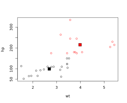
6. kmeans cars example

# The cars data frame is pre-loaded

# Set random seed. Don't remove this line
set.seed(1)

# Group the dataset into two clusters: km_cars
km_cars <- kmeans(cars, 2)

# Add code: color the points in the plot based on the clusters
plot(cars,col= km_cars$cluster)

# Print out the cluster centroids
km_cars$centers

# Replace the ___ part: add the centroids to the plot
points(km_cars$centers, pch = 22, bg = c(1, 2), cex = 2)